baSeq docs › Spatial transcriptomics

Spatial transcriptomics

A spatial analysis takes the genes of tissue sections counted where they are, from spots (Visium, Visium HD, Slide-seq, Stereo-seq) or from cells (Xenium, MERSCOPE, CosMx), finds the tissue's domains, its spatially variable genes, where each cell type is and which cells sit together, and lets you explore every section by hand.

Start a spatial analysis

In a project, click New session and choose Spatial Transcriptomics. The sidebar marks it with a section of tissue and its spots. Each tissue section is a sample: name it and give its condition in the panel that opens after the upload.

What to upload

Drop the platform's output folder, or a .zip of it. baSeq recognises the files by their names and content, also when GEO has given them a sample prefix (GSM5833536_A1_tissue_positions_list.csv.gz):

10x Visium (Space Ranger 1 to 4, CytAssist too): filtered_feature_bc_matrix.h5 (or its folder) with the spatial folder: tissue_positions.csv, scalefactors_json.json and tissue_hires_image.png.
10x Visium HD: the binned_outputs folder (the 8 µm bins are read when several sizes come), GEO's flat names (GSM1_square_008um_filtered_feature_bc_matrix.h5) or Space Ranger 4's segmented_outputs, read as cells. tissue_positions.parquet, scalefactors_json.json and tissue_hires_image.png put the bins on the section's image.
10x Xenium: cell_feature_matrix.h5 with cells.csv.gz or cells.parquet, and experiment.xenium, or the whole output zipped as 10x ship it. The negative-control probes and codewords are counted per cell and kept apart from the genes. The morphology_focus image of DAPI, when it comes, is drawn under the cells, dark on white.
Vizgen MERSCOPE: cell_by_gene.csv with cell_metadata.csv, also with the sample's name before or after them (cell_by_gene_SliceE.csv).
Bruker CosMx: the exprMat_file.csv with the metadata_file.csv, from the older exports and AtoMx alike.
Slide-seq and Curio Seeker: the counts with the bead locations (with a header or without), or Curio's .h5ad or its MoleculesPerMatchedBead.mtx with its barcodes, genes and MatchedBeadLocation.csv. A location file whose rows do not name their beads is refused with the reason.
Stereo-seq: a .gem or .gef file, or the same table as .tsv, summed into bin50 squares (25 µm).
Any .h5ad with spatial coordinates in obsm['spatial'], such as scanpy's and squidpy's Visium objects with their images.

Files the analysis never reads stay on your computer, or packed when they come in a .zip: every transcript on its own (Xenium's transcripts.parquet, MERSCOPE's detected_transcripts.csv), full image stacks, zarr stores and Visium HD's 2 µm bins. Spots and cells cannot be mixed in one session: they are analysed differently.

A single-cell reference

To map cell types, upload an annotated single-cell dataset of the same tissue with the sections: an .h5ad with raw counts and the cell types in a column such as cell_type. It is not a section: its types become profiles that Map Cell Types fits to every spot or cell. Without one, Map Cell Types finds programmes of genes (topics) instead.

The cell types in the reference are the ones you get. A type the reference lacks cannot be told: its cells go to the nearest types, with no warning (on a lymph node with germinal-centre cells removed from the reference, those spots became naive B cells and macrophages, with no loss of confidence). So choose a reference that covers the tissue. Types in the reference that the section does not hold do no harm: breast tumour types added to a lymph node's reference took 0.2% or less. Shares are best compared for one type across the tissue: between types they depend on how much RNA a cell of each type gives. On an imaging panel, fewer than about 100 genes shared with the reference is too few to trust one type per cell (real Xenium: 75% right at 250 genes, 54% at 60), and the figure says so.

Which column holds the types: baSeq takes a known name (cell_type, celltype, annotation, subclass and others), says which it took and which others could hold types. To use another, name it cell_type in the file. Labels that are no cell type (low quality, unknown, unlabelled, doublet, hybrid) are left out and listed, because as profiles they take in the cells they resemble.

Spots, bins and cells

Every platform's positions are converted to micrometres, so distances, neighbourhoods and scale bars mean the same for every section. What a row is decides the defaults: a Visium spot holds a few to a dozen cells, so its cell types are a mixture and its quality is judged against the spots around it; a Xenium cell is one cell, judged by its transcripts, negative controls and area. Neighbours are the touching spots on Visium's grid and the Delaunay neighbours of cells, and they never cross from one section to another.

Tissue Quality Control: counts, genes and the mitochondrial share drawn on a Visium section of a human lymph node, with the spots out of line with their neighbours in red — Tissue Quality Control on 10x's human lymph node: the measures where they are, and the few spots out of line with their neighbours (red). The band of higher mitochondrial share stays: its spots match each other.

Domains, cell types and niches

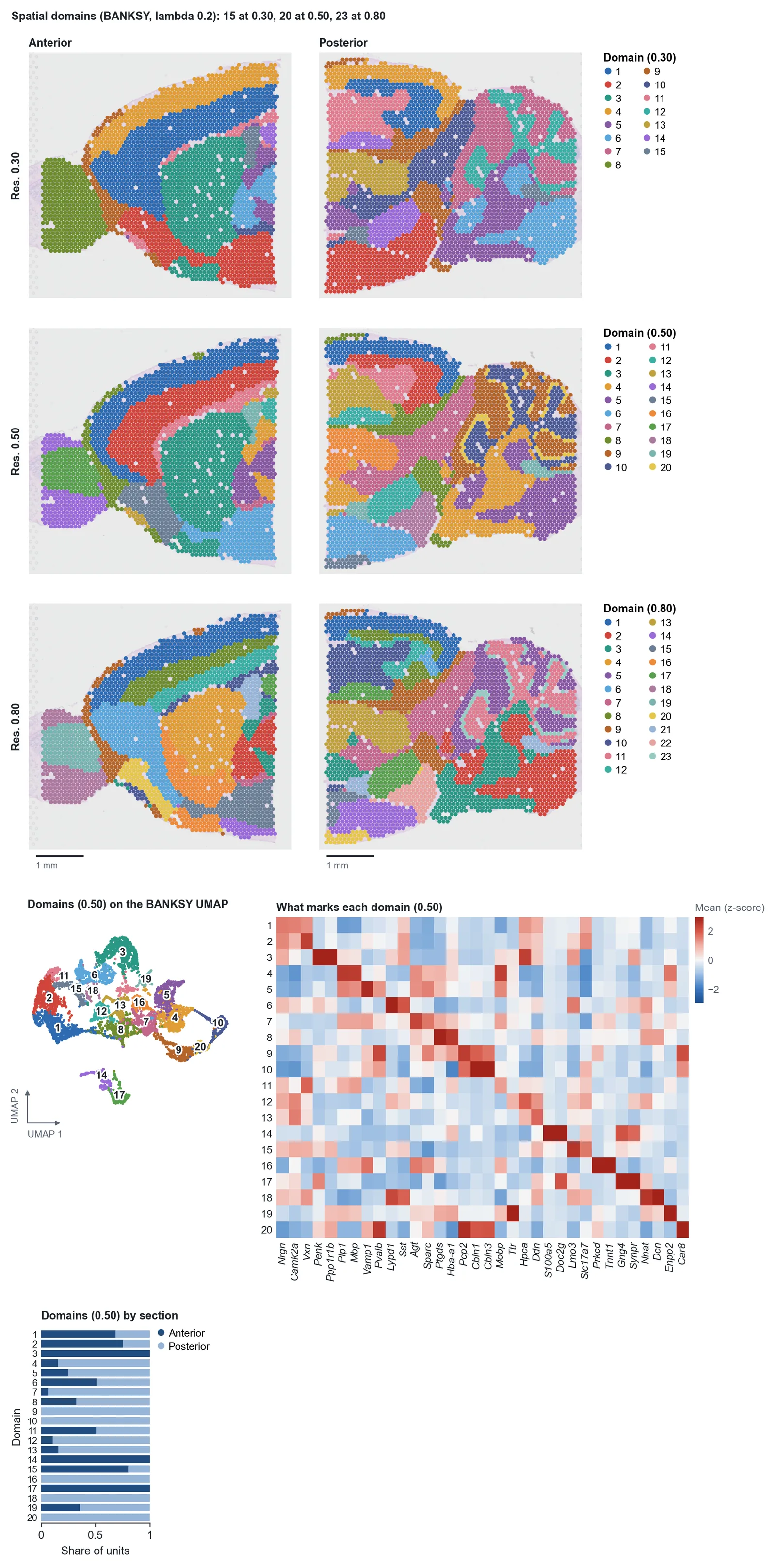
Spatial Domains clusters each spot or cell on its own expression and its neighbours' (BANKSY), so regions of tissue come out whole where clustering the expression alone scatters them, and a domain has one number in every section. The figure ends with the genes that mark each domain, to name them by.

CosMx and MERSCOPE image a section field by field, and on real sections that can show. If neighbours differ far more often across a field's edge than the same distance apart inside one, or a domain gathers along the fields' edges, where counts fall, the step finds its domains again with Harmony on the fields, or on the distance from their edges, and says so over the figure. A whole field that is a domain by itself is named there and left alone: a large structure can fill a field too. Correct imaging fields can be set to always or never. The expression's clusters do not split at fields, and are not corrected.

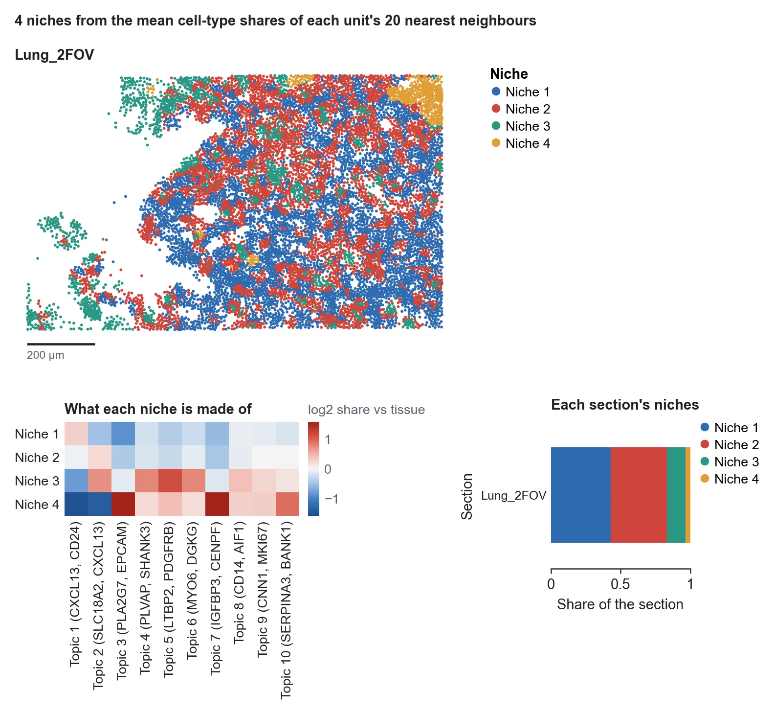
Spatial Domains: BANKSY domains at three resolutions on the two halves of a mouse brain section, the BANKSY UMAP, the genes that mark each domain and the domains by section — Spatial Domains on 10x's mouse brain, the two halves of one sagittal section: the olfactory bulb, the cortex in its layers, the striatum, the hippocampus, the thalamus and the cerebellum come out as domains, with one number across the two halves.

Map Cell Types places the reference's cell types (or topics without one), and Cellular Niches groups spots or cells by what surrounds them: the make-up of each niche against the tissue as a whole, and how much of each section each niche takes, so a niche that comes with a condition stands out.

Cellular Niches on a Xenium section of human lung: the niches on the tissue, what each is made of, and the section's share of them — Cellular Niches on 10x's Xenium human lung, from the programmes of genes around every cell: the epithelial mass, the stromal and vascular islands within it and the region of another epithelium at its corner.

Exploring the tissue

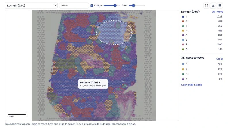
Every result of a spatial session has an Explore tab beside its figure: the sections drawn as they are, to look around by hand. Scroll or pinch to zoom and drag to move; it stays smooth with a million cells. Colour the tissue by any grouping (clusters, domains, cell types, niches, sections), any measure (counts, QC, module scores, each cell type's share) or any gene: type its name. The section's image lies under the spots and can be faded. Click a group in the legend to hide it, double-click it to see it alone; hover to read what is under the pointer; hold Shift and draw around a region to count what it holds, and copy the names of its spots or cells. The colours are those of the step's figure. The view can be saved as a PNG or opened full screen.

The Explore tab: a Visium section of a human lymph node over its H&E image, coloured by domain, with a region drawn around and the composition of its spots — The Explore tab on 10x's human lymph node: its domains over the H&E image, a region drawn around with Shift (what its spots hold listed at the right) and the spot under the pointer.

Ligand-receptor pairs: what they can and cannot show

Ligand-Receptor Pairs ranks the curated pairs your data measures by how much they overlap in the tissue: the receptor in each spot or cell times the ligand around it, within about 100 µm for a secreted ligand and about a unit's width for one that needs contact. The Explore tab can then colour the section by the activity of each of the top pairs.

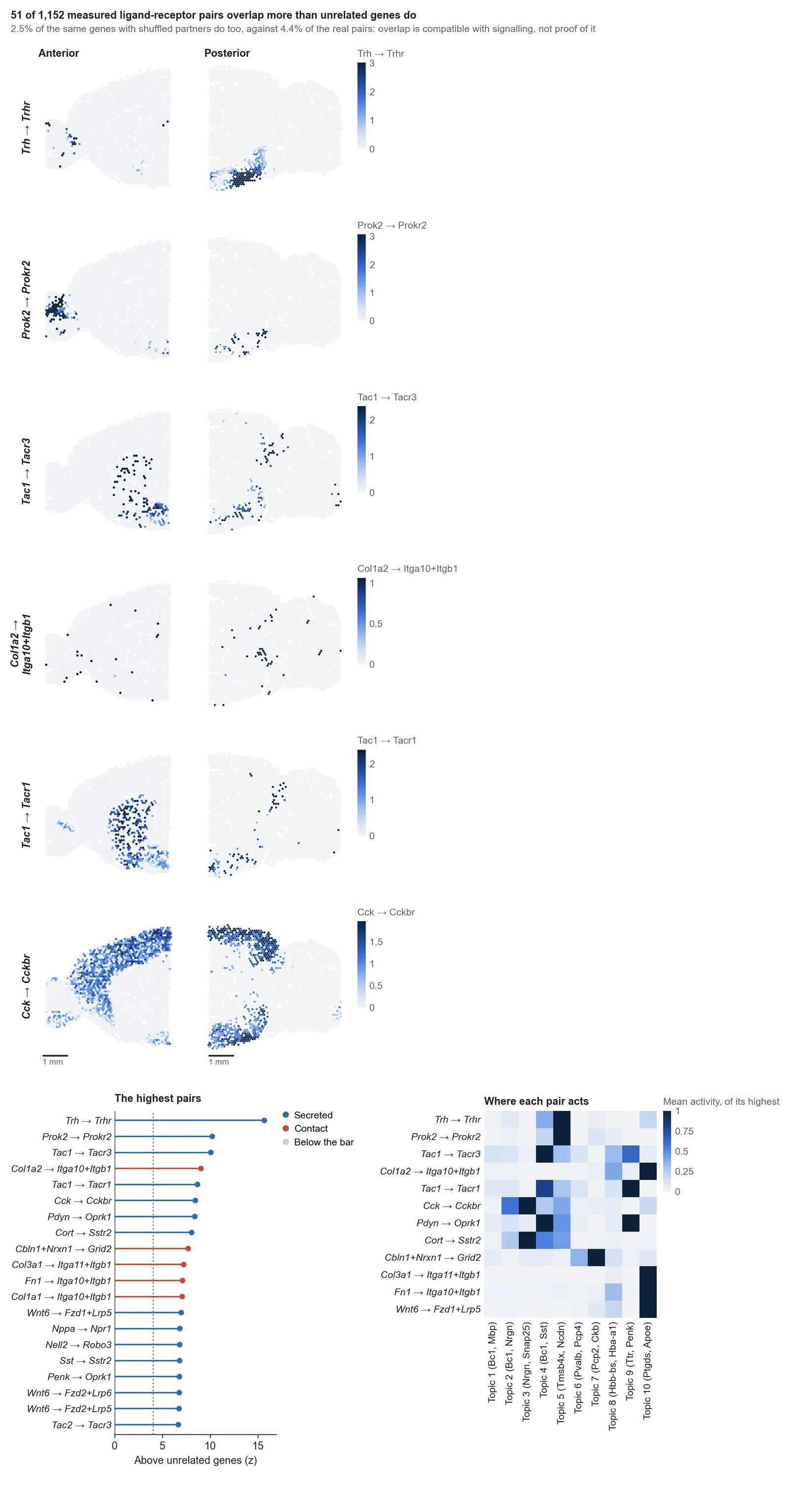
Ligand-Receptor Pairs on a Visium section of a mouse brain: the top pairs on the tissue, the ranking and where each acts — Ligand-Receptor Pairs on 10x's mouse brain, without being told any anatomy: Tac1 to Tacr1 in the striatum, Cck to Cckbr in the cortex and hippocampus, Prok2 to Prokr2 in the olfactory bulb. The note under the heading gives how often shuffled partners reach the same bar.

Overlap is compatible with signalling. It is not evidence of it

Genes of one compartment overlap whether or not their proteins bind. So the figure also reports how often the same genes with their partners shuffled pass the bar. On a lymph node 3.9% of the real pairs pass and 1.8% of the shuffled ones; on a mouse brain 4.4% and 2.5%. That is, about half of what stands out would stand out with the wrong partner, and fewer at the top of the list. Read the ranking as a list of pairs to look at and confirm by another means.

A pair whose sender and receiver sit in separate compartments reads as apart: LTB with LTBR and CD40LG with CD40 do not stand out on a lymph node, though they act there. A gene panel holds both partners of few pairs (8 of 1,730 on Xenium's 289-gene lung panel), and then the figure says so and calls nothing.

Why not the usual test: comparing the overlap with shuffled spots, as most tools do, flagged 22% of housekeeping genes and of random gene pairs on the real lymph node, because two genes with any pattern overlap far more than two shuffled ones. Here a pair is compared with pairs of unrelated genes with the same detection. Under 1% of housekeeping and random pairs reach the bar, and the score hardly follows expression. Pairs of proteins only: where a database lets a synthesis enzyme and a transporter stand in for a small molecule such as glutamate, that is not a measurement of the ligand.

The methods

baSeq follows the field's current practice. BANKSY led the benchmarks of its paper for both domain segmentation and cell typing and scales to millions of cells without a GPU; its settings follow the platform, as its authors recommend. Moran's I is the reference test for spatially variable genes and is as good as the newer ones in independent benchmarks. Reference-based mapping with platform effects (RCTD's approach) led the benchmarks of spot deconvolution. Quality control compares each spot with its neighbours rather than with the whole section, as SpotSweeper does, so tissue that simply holds less RNA is not thrown away. The single-cell steps (annotation, markers between clusters or domains, pseudobulk, heatmaps, violins, GSEA, STRING, pathway maps) run on the spatial data as they are.

Step reference

Step	Stage	What it does	You get	Key inputs
Initial Plot	Setup	Reads every section, whatever platform made it, places each spot, bin or cell in micrometres, keeps the section's image, and turns a single-cell reference uploaded with the sections into cell-type profiles.	Each section with its counts where they are over its image, the spots or cells per section, the top genes, and a table of the sections.	None.
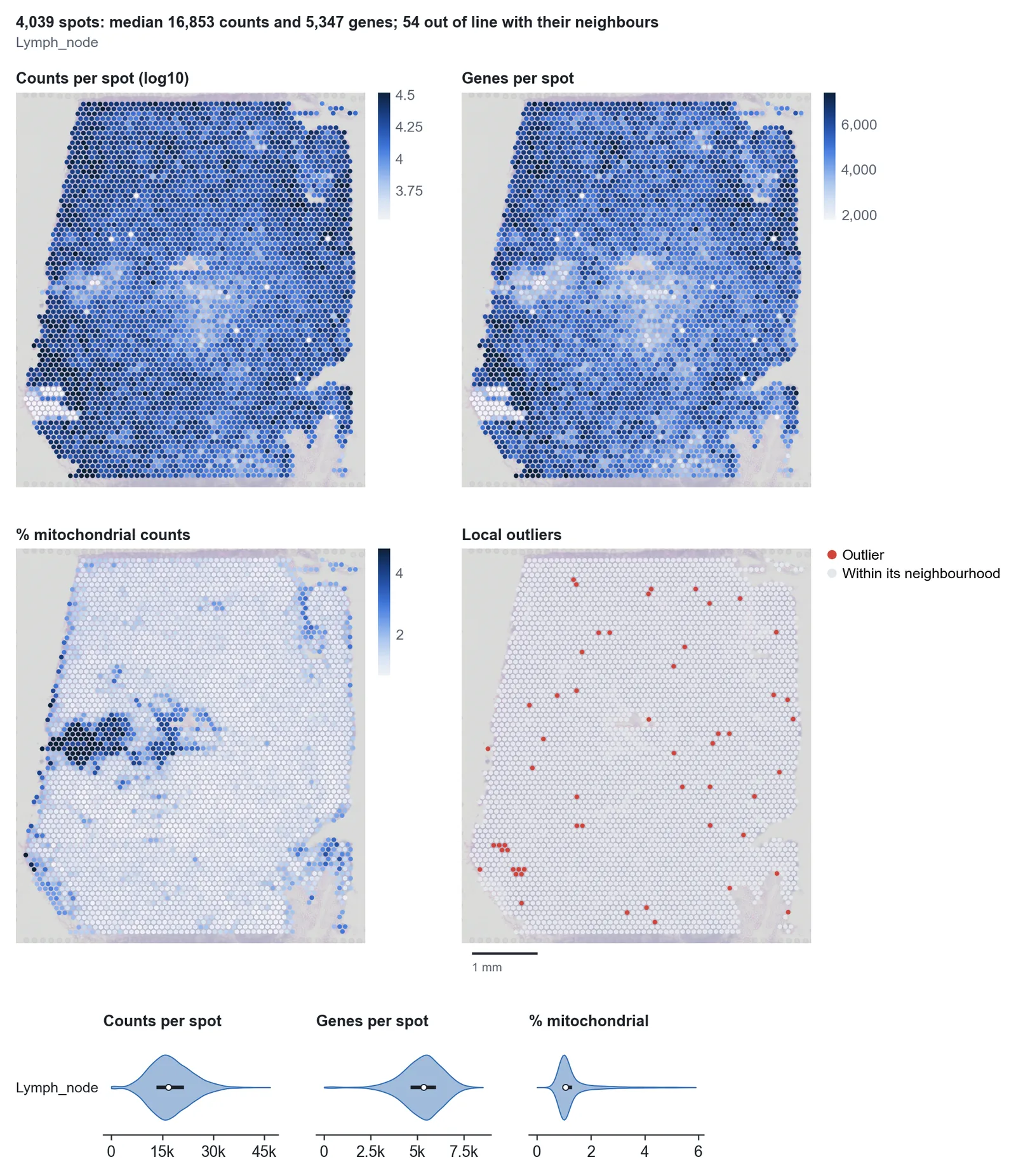
Tissue Quality Control	QC	Counts, genes, the mitochondrial share and, for imaging panels, the negative-control share and the cell area of every spot or cell, drawn where they are. Each spot is also compared with its 36 nearest spots (SpotSweeper, Totty et al. 2025).	The measures on every section, the spots out of line with their neighbours, and violins per section.	None.
Quality Filtering	QC	Spots: removed when far below their own neighbours (a whole region of low counts stays, because it is more often tissue than a fault), when their mitochondrial share is above both their neighbours' and 5%, or under a floor. Beads: the floor is the dip between the shallow beads off the tissue and those on it, when their counts have those two modes. Cells: removed with few transcripts, many negative-control counts or an unusual area (segmentation fragments and merged cells).	Where the removed spots or cells were, by reason, the counts kept per section, and a note when separate pieces of tissue fare differently, as one floor can take most of a piece with little capture.	Approach, distance from the neighbours, minimum counts and genes, maximum negative-control share.
Normalize Data	QC	Library size and log (standard), cell area and log, which keeps how much RNA a cell holds (Atta et al. 2024), or Pearson residuals for PCA. The size factors are drawn on the tissue: where they follow its structure, normalising by them takes some of that structure away (Bhuva et al. 2024). Where depth varies across a section, as at a fold, cell area leaves it in, and PCA says so.	The size factors on every section, and the counts before normalising.	Normalisation.
Highly Variable Genes	QC	The genes that vary most beyond their mean (Seurat v3 on the counts, per section); a targeted panel of up to 1,000 genes is used whole. Mitochondrial and ribosomal genes are left out, and genes found in under 0.2% of the units, whose few stray counts Seurat v3 ranks high on sparse bins and beads.	Every gene's variance against its mean, the chosen ones named.	Number of genes.
PCA	QC	Principal components of the highly variable genes. Those above noise go on to integration and clustering, by parallel analysis (each gene shuffled on its own gives the noise's level), and at least 20: a small panel at low depth has few, and the others only give clustering noise to cut.	The variance explained against the noise, and the first four components on the tissue, where a fault (a slide edge, a dry patch) shows before clustering; a component that follows the counts says so.	None.
Perform Integration	QC	Harmony, Scanorama or scVI across sections, as in a single-cell analysis.	UMAPs before and after.	Method.
Clustering	Analysis	Leiden clusters of the expression at resolutions 0.30, 0.50 and 1.00, each drawn on the UMAP and on every section in the same colours.	The clusters on the UMAP and the tissue, and, with several sections, the clusters by section.	None.
Spatial Domains	Analysis	BANKSY (Singhal et al. 2024): each spot's or cell's expression together with its neighbours' mean and how expression changes across the neighbourhood. The settings follow the platform, as BANKSY's authors give them: lambda 0.2 and two rings of spots on Visium, whose spots already average several cells; lambda 0.8 on the high-resolution platforms. Sections are aligned with Harmony when there are several batches, so a domain has one number in every section, and a difference between conditions is read within it. Then Leiden at three resolutions, borders smoothed, specks joined to their neighbours. On CosMx and MERSCOPE the imaging fields are integrated too, when the domains are seen to split at their edges.	The domains on every section, the BANKSY UMAP, the genes that mark each domain (those furthest above the next highest domain, saying which domains hold far fewer counts), and the domains by section.	Neighbourhood weight (lambda), smoothing, imaging fields.
Spatially Variable Genes	Analysis	Moran's I of every gene found in at least 0.1% of the spots or cells, on the neighbour graph, with the randomisation variance and Benjamini-Hochberg; a gene counts from I 0.02, as with this many units a significant I can be next to nothing. Mitochondrial and ribosomal genes are tested but not ranked; the strongest other genes are grouped into modules that share one pattern.	The top genes and the modules drawn on the tissue, the strongest genes ranked, and tables of every gene and module.	False discovery rate, number of modules.
Map Cell Types	Analysis	With a single-cell reference: each gene's platform effect estimated first (as RCTD), then each type's share in every spot, or the one most likely type of every cell. Without one: topics (LDA, as STdeconvolve) of the most variable genes, mitochondrial and ribosomal ones left out.	The largest type and each type's share on the tissue (or the type and its confidence per cell), and the types by domain.	Spots or cells, number of topics.
Neighbourhood Enrichment	Analysis	How often two groups touch, against the labels shuffled 1,000 times within each section and each separate piece of tissue in it (squidpy's test, shuffled more narrowly), and how co-occurrence changes with distance.	The groups on the tissue, a z-score heatmap, and the closest pairs over distance.	Groups.
Cellular Niches	Analysis	Each spot's or cell's surroundings (the share of each type among its nearest neighbours), grouped into niches (Schurch et al. 2020).	The niches on the tissue, what each is made of, and how much of each section it takes.	Groups, neighbourhood size, number of niches.
Ligand-Receptor Pairs	Analysis	How much each curated pair (CellPhoneDB v5, proteins only) overlaps in the tissue: the receptor in each spot or cell times the ligand around it, against unrelated genes of the same detection and against the same genes with their partners shuffled.	The top pairs on the tissue, the ranking, where each pair acts and which groups express each partner.	Groups, which pairs, the reach of a secreted signal.
Explore Genes on Tissue	Analysis	The genes you name or describe, drawn on every section on one scale per gene, beside violins by domain.	Each gene on every section, and the genes by domain.	Your description; violins by.

Checked on real tissue and on planted data

Every step has run on three of 10x's public datasets and every figure has been looked at. On the human lymph node (Visium) the domains and the gene modules separate plasma cells, follicles, germinal centres, the T zone and a patch of interferon response, each marked by its known genes. On the mouse brain (Visium) the domains follow the anatomy across the two halves of the section. On the human lung (Xenium) modules of T and NK cells and of dividing cells come out from a panel of 289 genes at 56 counts per cell; with half the cells as a reference, labelled by Xenium's own clusters, the other half were mapped to the right lineage 81% of the time.

With real references from separate experiments, Map Cell Types was scored against what others published. On the lymph node, with the cell2location paper's reference, each type's map agrees with that paper's cell2location and RCTD results (median r 0.68 and 0.77; they agree with each other at 0.74), and manual germinal centres are found better than by either (AUC 0.990 against 0.979 and 0.967). On a mouse brain each type's map agrees with the published one at r 0.91. On Xenium breast cancer with a Chromium reference from another patient, 75% of cells get the right coarse type, on labels made without that reference.

The other platforms have run through the same steps on public data, with every figure read against the tissue's anatomy. CosMx (two slides of human colon, an older export and AtoMx): crypts, the lamina propria's plasma cells, muscularis mucosae, submucosa and surface epithelium, and follicles on the slide that has them. MERSCOPE (a mouse brain, a human fetal gut): CA1 by Fibcd1, white matter, meninges and dopaminergic neurons; epithelium and mesenchyme. Visium HD (a mouse kidney, 8 µm bins over its image, a crop of 100,001 of 456,334 bins): proximal tubule, thick ascending limb, inner stripe, papilla, urothelium and smooth muscle in their order. Stereo-seq (half a mouse brain, whose .gem and .gef give the same counts in every bin, and an olfactory bulb): cortex, hippocampus, thalamus, hypothalamus, striatum, habenula and white matter. Slide-seqV2 (a mouse kidney): the proximal tubule's three segments, distal tubule and glomeruli. Curio Seeker (a mouse lymph node): T zone, follicles, fat and the medulla's macrophages.

What these do not settle: the cortex's layers do not come out as domains on Stereo-seq at the standard settings; a domain's straight edge can rest on a real gap in a Stereo-seq chip, where expression does not jump, and is then a gradient rather than a border; a section's pieces with very different capture split its domains by piece, as on the fetal gut, whatever the tissue; and without a reference, topics on sparse bins and beads include noise, and their names are their top genes only.

The test suite runs the pipeline on four Visium sections and two Xenium regions made with known answers: tissue domains of known make-up, a gene that rises across the section, spots far below their neighbours, a region of low counts, segmentation fragments and noisy cells.